Kyle Corry

Cloud Image Classification on a Smartphone

2022-10-01

Clouds have long been used as indicators for weather prediction. Having an accurate historical log of cloud types can be helpful in forecasting the passing of weather fronts, especially when combined with barometer data over time. In this article, I'll cover the system used in Trail Sense, which allows for offline classification of the 10 main cloud genera using a smartphone camera with minimal processing requirements.

Background

Cloud genera

Clouds are classified into 10 main genera based on their appearance and altitude. The 10 main genera are as follows:

• Cirrus (Ci): Thin, wispy clouds that form at high altitudes
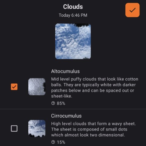
• Cirrocumulus (Cc): Small, puffy clouds that form at high altitudes
• Cirrostratus (Cs): Thin, sheet-like clouds that form at high altitudes
• Altocumulus (Ac): Puffy clouds that form at mid altitudes
• Altostratus (As): Sheet-like clouds that form at mid altitudes
• Stratocumulus (Sc): Puffy clouds that form at low altitudes
• Stratus (St): Sheet-like clouds that form at low altitudes
• Cumulus (Cu): Puffy clouds that form at low altitudes
• Cumulonimbus (Cb): Puffy clouds that form at low altitudes and can produce precipitation
• Nimbostratus (Ns): Sheet-like clouds that form at low altitudes and can produce precipitation

It is common for manual classification of clouds to use factors such as color (dark gray, white, see through), texture (smooth, puffy, wispy), and shape (wisps, sheet, clumped). An automated classification process should focus on trying to quantify these factors.

Not all of these cloud types are equally common, which can make data collection difficult and lead to an uneven distribution of data.

Gray-Level Co-occurrence Matrix (GLCM)

A Gray-Level Co-occurrence Matrix (GLCM) is a matrix that describes the spatial relationship between pixels in an image. The matrix is constructed by counting the number of times a pixel with a certain value and its neighbor with a certain value occur in a given direction. The resulting matrix can be used to extract texture features from the image. [2]

Logistic Regression

Logistic regression is a classification algorithm that uses a softmax function to classify an input into one of several classes. The softmax function is defined as follows: softmax(x) = exp(x) / sum(exp(x))

This algorithm is easy to implement, relatively fast to run, and does not require a large memory footprint. It is also easy to interpret the results of the algorithm and see how it decided upon the classification.

Solution

The following steps outline the process of classifying a cloud image:

1. Resize the image to 400x400 pixels. This reduces the memory footprint and improves the performance on low-end devices.

2. Calculate the average Normalized Red-Blue Ratio (NRBR) of the image. The NRBR is calculated as [1]: max(1, (red - blue) / (red + blue))

3. Calculate the normed, symmetric 16 level Gray-Level Co-occurrence Matrix (GLCM) of the red channel for each 100x100 region of the image using the following step sizes (averaged): (0, 1), (1, 1), (1, 0), (1, -1). [2][3]

4. Compute the following features for each GLCM and take the average of each feature across all the GLCMs [3]:

   • Energy
   • Contrast
   • Vertical Mean
   • Vertical Standard Deviation

5. Normalize each feature as follows:

   • NRBR: Map it from the range [-1, 1] to [0, 2]
   • Energy: Take as is
   • Contrast: Take as is
   • Vertical Mean: Map it from the range [0, 16] to [0, 1]
   • Vertical standard deviation: Map it from the range [0, 3] to [0, 1]

6. Feed all features, plus a bias of 1 into a logistic regression classifier.

Results

After training on a small dataset (~300 images) that was unevenly distributed, the weighted average F1 score was 0.63. On the more common cloud types, it performed a bit better (Cu: 0.8, Ac: 0.76, Ci: 0.67, Sc: 0.67). With more training data (and better distribution), I believe this score will improved.

This solution should act as a starting point for further research into cloud classification on a smartphone. It is not perfect, but it is generally accurate on the common cloud types and is able to run on a lower end smartphone in real time.

This model was included in version 4.6.0 of Trail Sense.

References

1. Heinle, A., Macke, A. & Srivastav, A. (2010, May 6). Automatic cloud classification of whole sky images. Retrieved from https://doi.org/10.5194/amt-3-557-2010
2. Hall-Beyer, M. (2017, April 4). GLCM Texture: A Tutorial v. 3.0. Retrieved from https://doi.org/10.11575/PRISM/33280
3. Brynolfsson, P., Nilsson, D., Torheim, T., Asklund, T., Karlsson, C., Trygg, J., Nyholm, T. & Garpenbring, A. (2017, June 22). Haralick texture features from apparent diffusion coefficient (ADC) MRI images depend on imaging and pre-processing parameters. Retrieved from https://doi.org/10.1038/s41598-017-04151-4